
Research summary: Perthes’ disease and cartilage stress
In the last publication from my PhD thesis, I made a “digital twin” finite element model of the hip to predict damaging stresses in the cartilage during walking. I demonstrated this by simulating both hips in a single patient with Perthes’ deformity—one side affected and the other unaffected. The results of this demonstration showed the importance of considering not just the forces applied to the hip but also its motion, and similar techniques could be used to tailor patient-specific surgical or non-surgical management pathways for patients with residual Perthes’ deformity.
The full paper is available open-access in the International Journal of Computer-Assisted Radiology and Surgery as:
The meta-story
What? Another paper from my PhD? I’m as surprised as you are—this one was never part of the PhD plan. Most of the chapters in my thesis, covered in previous research summaries, were about measuring features and outcomes of Perthes’ disease that could be measured using MRI scans. My advisory committee, however, thought I should do more to show off my engineering chops, being in an engineering program and everything. Fair enough!
This led me to add in a little chapter with some very engineeringy computational modelling, a simple proof of concept using a 3D reconstruction of both hips from one of my MRI participants. This participant had unilateral Perthes’ deformity, so we could compare stress in the articular cartilage (the low-friction joint tissue that degrades during osteoarthritis) between the affected and unaffected sides.
I was pointed towards a platform called ArtiSynth for my modelling and soon found myself part of a small and friendly community of users. Despite the steep learning curve, it was very convenient to have the developers based in UBC and keen to give support. One thing led to another and I was presenting my early model at a special session of the CMBBE conference in 2024. People seemed to like it!
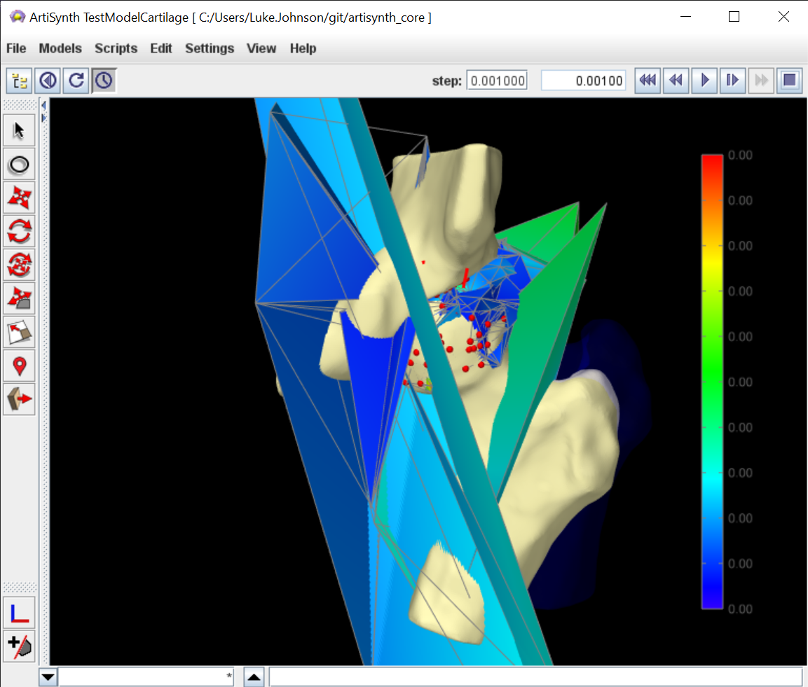
An early simulation attempt that ended in catastrophic failure. Better tweak my constraints!
Fast forward to January 2025 and my post-PhD limbo period. There were about three months between defending and graduation with minimal thesis revisions required (look at Dr Clever Clogs here). So, hey, why not just quickly write up1 this last chapter and throw it at a journal we’ve had a good experience with? To make it more of a rounded study I added some more rigorous sensitivity analyses2 and a look at predicted hip stresses in high flexion postures (imaged during the study on hip clearance in Perthes’).
So without any further ado, here’s what it’s all about.
Why study this?
In an earlier study, we linked the shape of residual hip deformity after Perthes’ disease with painful hip impingement, which could contribute to worsening cartilage health in Perthes’ hips during adolescence and young adulthood. By using an upright open MRI we could see hip impingement in vivo3, but only in a small number of static positions. This gives us an incomplete picture of what happens in the hip during typical daily activities like walking.
The MRI also doesn’t provide any information about the stress experienced by the hip joint’s cartilage; shear stress in particular is known to play a key role in cartilage damage. Computational tools like finite element models can predict cartilage stress, but so far haven’t been used to study how the hip’s motion interacts with its shape to cause damaging stress concentrations in Perthes’ deformity.
What I did
As we can see below, there was a lot that went into this model. In brief, I took the shape of the hip joint bone and cartilage from one patient’s MRI scans and combined it with motion and forces representing a “typical” walking pattern from previous studies by other groups. The model then takes these inputs and simulates a complete walking step from one point where the foot first touches the ground to the next.
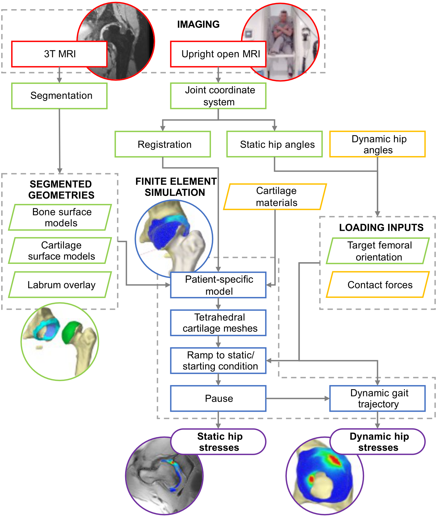
A lot of data was brought together from MRI sources (red) and analysis (green), as well as from the literature (yellow). These were brought together in the ArtiSynth model (blue) to find an estimate of shear stress distribution in the hip joint cartilage (purple).
The forces applied to the ball of the femur bone (the femoral head) are distributed in the form of stress through the cartilage, and the model tracked the highest shear stress on the femur and pelvis sides of the joint over time.
A big advantage of this model is that it’s not just limited to studying walking—it’s designed in a way that any arbitrary motion and force profile can be used. Taking advantage of this, I also wanted to see how well the model could represent extreme postures, such as those in our earlier upright MRI impingement study. I was able to calculate the exact position of the joint from this patient’s images as well as the orientation of the imaging plane in each posture, which were then used as inputs to the model.4
What I found
The results of the walking simulation sort of speak for themselves—there were generally higher stresses in the affected hip that had had Perthes’ compared to the other side, particularly in the early parts of the gait cycle.
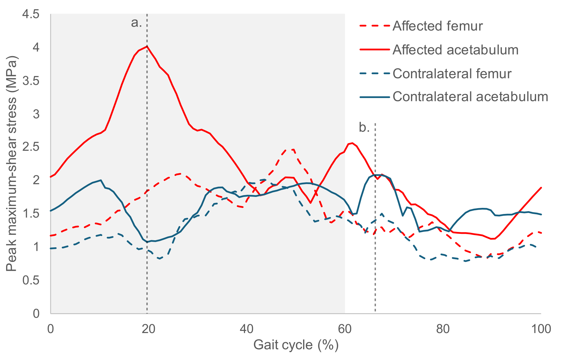
The highest stress in the affected (red) and unaffected (blue) hips, plotted across a typical walking cycle. The shaded region in at the start is when the foot is placed on the ground (the “stance phase”) during which the loads on the hip are highest. There is a notable shear stress peak in the affected hip socket (acetabulum) during at 20% gait, while the peak in the unaffected side is at 67% gait.
One very important observation is the importance of the joint’s position as well as the strength of the input force. Most previous research using similar methods to study hip joint stress pick a single moment in time to simulate, based on when the forces are strongest. This is likely a reasonable approach when the hip joint is well rounded, but in Perthes’ the motion of the highly aspherical femur could cause stress concentrations at any time.
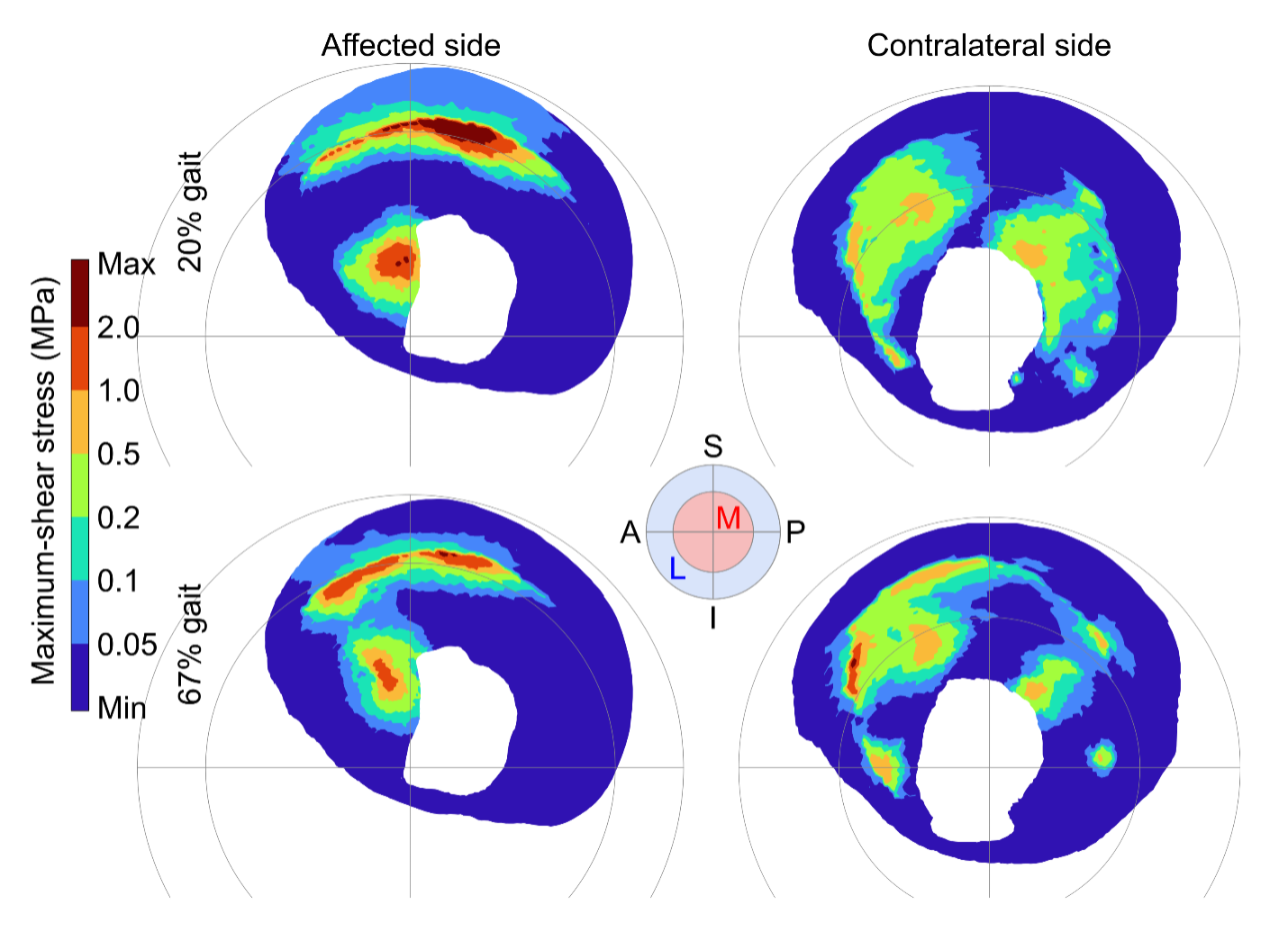
The stress distribution in both hip sockets the key time points indicated with dashed lines in the previous figure: 20% and 67% gait.
In my simulation of more extreme joint postures, the model did an excellent job of matching the in vivo position of the bones seen on MRI, as shown by cross-sections overlaid on the MRI slices below. Stress concentrations were also located at the rim of the hip socket, consistent with our expectations.
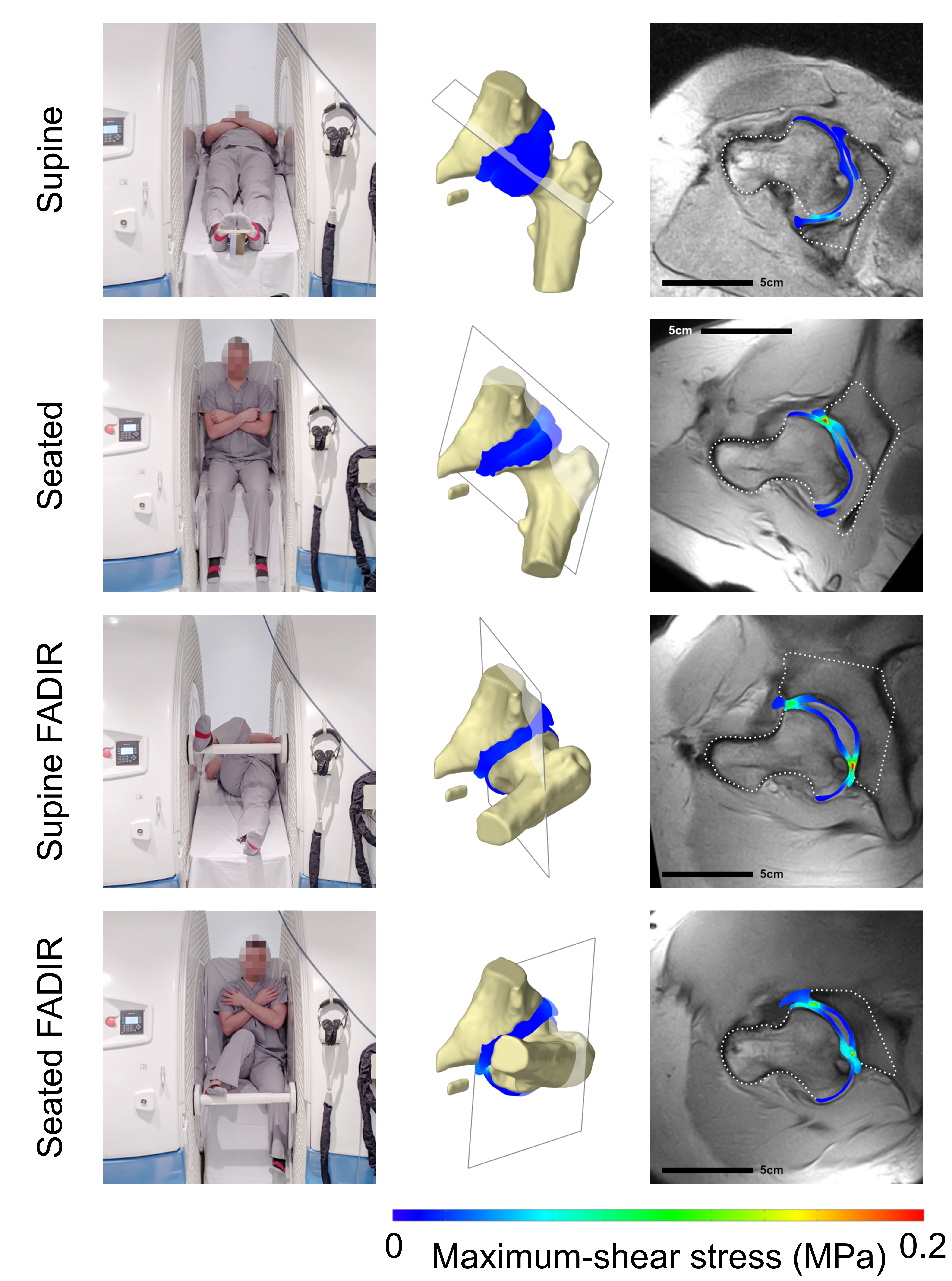
I simulated the hip in high flexion postures to match positions scanned in the upright open MRI (left: postures demonstrated by a healthy volunteer). Cross-sections of the stress distribution are overlaid onto the MRI slice (right).
One area for future work is to make the model more robust to changes in the input parameters. For example, small differences in the orientation of the hip—about the same size as the typical error from motion capture—had a big impact on the stress outputs. This kind of sensitivity would be a major limitation for future applications, but there are plenty of ways it could be tackled, such as improvements to surface preparation or use of a more robust outcome measure than overall peak stress.
Stuff I wished I could talk about
This section is a more technical! Feel free to skip it if you’ve never done any finite element analysis before.
Here’s the bit where I really go into how the sausage was made. It’s a lot uglier than the polished final product might suggest, and there were some major trade-offs that were needed to get a dynamic model to run in a reasonable time on a reasonably-powerful computer. In the end there’s only so much you can put in a research paper, so here are two of the things that didn’t make the cut.
One detail that may catch the attention of any finite element experts is the use of linear tetrahedral5 (tet) elements for a stress analysis in a nearly-incompressible material. Normally this is a big no-no! This is because they are susceptible to “volumetric locking”, resulting in the material acting much stiffer than the nominal material properties.
However, there are three reasons why I decided to stick with linear tets:
- They’re very easy to generate from our starting point of a triangular surface mesh. This functionality is built into ArtiSynth, whereas generating a hexahedral mesh requires additional software and complication.
- Linear tetrahedral elements are fast. The time step for our simulations was 0.002 seconds, so speed was of the essence.
- The exact stress value isn’t critical. I’m not trying to design a bridge here, where incorrect estimates could put lives in danger. My focus is more on the relative magnitude of stress between healthy and Perthes’ hips, and the location of stress concentrations.
To justify these arguments, I ran some preliminary tests in which a solid ball was pushed into a thin rectangular block of “cartilage” made up of linear tet, quadratic tet or linear hex elements. The block was meshed with one, two or three layers of elements. With more than one layer, the linear tet meshes overestimated cartilage stress by a consistent 17-18% compared to the corresponding hex meshes6—and ran twice as fast—so I added a step in the ArtiSynth code that ensured there was always at least two element layers in thin cartilage regions.
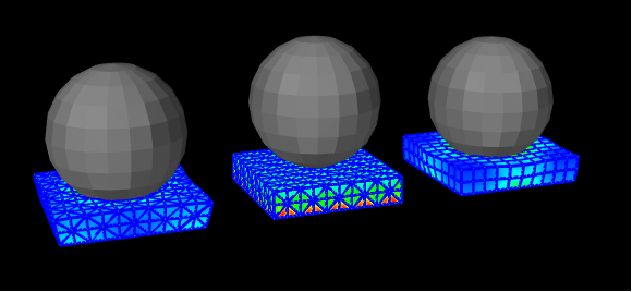
An early version of the preliminary indentation tests to compare different element types. The “bulging” of the sides seen here isn’t too representative of real hip cartilage, so I eventually added constraints to limit this.
I used peak stress over time as the variable of interest, mainly to make it easier to compare with previous studies. However, I’m not sure if it’s the right idea for future work. Peak stress is vulnerable to outliers caused by the discretisation of a smooth tissue into angular blocks, an effect compounded by the motion of the model, so it was challenging to reach a converged mesh.7 In addition, the absolute peak stress is extremely unrepresentative of the rest of the cartilage—even of the top percentile of nodes in the mesh! If we want a better idea of the mechanical environment in the joint it might be worth considering regional averages, using the 99th percentile stress to represent the “high stress region”, or defining a damaging stress threshold and measuring the proportion of tissue that is above it.
Wrapping up
I learned a lot from this study and it was good fun to put together. Also, it is definitely the most aesthetically pleasing of my papers so far! However, the model was always intended to be a proof-of-concept so I can’t really draw many important conclusions at this point. There are plenty more improvements that could be made before any future research or clinical application, but the probable best use-case would be as an initial rough estimation of shear stress concentrations, to then be confirmed with more accurate models. This approach could be helpful to identify “at-risk” motions for patients to avoid, or to help surgeons assess range of motion during preoperative planning.
-
Nothing is ever “just a quick write-up”. Ever. ↩︎
-
A sensitivity analysis is where you change some of the model’s inputs or properties to see how much the outputs change. It’s useful to determine how accurate your inputs your need to be or if it’s ok to use rough estimates. ↩︎
-
Studying something in a living organism, as opposed to studying a body part taken from a cadaver (ex vivo) or cells/tissues grown in a lab environment (in vitro). ↩︎
-
For this part of the study we also changed the material properties of the hip joint’s cartilage, i.e. how squishy it is. Cartilage is stiffer when it is loaded quickly, so for the walking simulation we defined properties representative of repeated loading and unloading every second. In the MRI, the patients were holding the same position for 20-30 minutes, so a much softer material was used to represent a constant load. ↩︎
-
Triangle-based pyramid. ↩︎
-
The quadratic tet meshes were very unstable, likely due to issues with contact mechanics, but when I could get them to run they performed similarly to the linear hex meshes. ↩︎
-
A finite element mesh is considered converged when increasing the number of elements (the mesh density) no longer meaningfully changes the output. The linear tets probably didn’t help with this either. ↩︎
Comments
You can use your Mastodon or other Fediverse account to comment on this post by replying to this thread.
Alternatively, you can reply to this Bluesky thread using a bridged Bluesky account.
Learn how this is implemented here.